Scale Dependent Convolution layer
Dealing with scale with parametrized dilated convolution
Motivation
Image analysis pipelines based on the segmentation, extraction of features of interest and aggregation of this information for subsequent prediction, allow for apriori and aposteriori analysis in addition to being more “trustworthy”. Indeed as the model is build around objects selected by experts, predictions can be traced back to these elements, thus increasing the trust and interpretability.
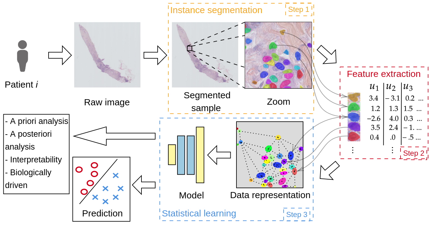 Figure 1: Random samples from the dataset
These models are particularly useful for large image data when the amount of information is enormous and the probability to over-fit very high. Fields such as bioimaging and remote sensing can benefit. However the object we segment and extract from can have very different sizes. To overcome this difficulty, we propose a Scale Dependent Convolutional layer in order to take into account different sizes while operating on resized objects.
Main idea
NN have benefited from batch sampling, with batch gradient descent and batch layer normalisation, to obtain state of the art results. However, when object are of a different size, there are two options:
- ignore the scale by resizing all input images
- crop a larger window than most objects
The second option has some limitations has depending on the range of the objects, the window could be insufficient or the object too small. Based on the dilation convolution we propose to parametrize the convolution layer in order to adapt the dilation to the actual size.
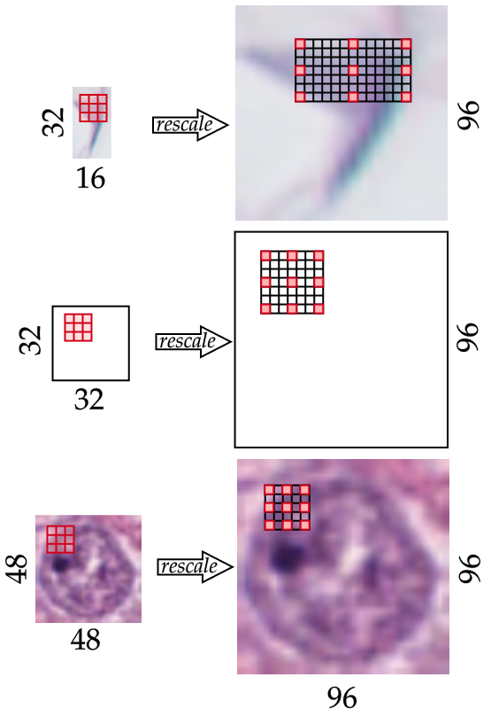
Figure 2: Scale Dependent Convolutional Layer – SDCL
We give below the equation for our parametrized dilated convolution for computing the resulting feature map $m$ at pixel $(i_0, j_0)$ for a one channel input image: \(f_m^{sd}(I)[i_0, j_0] = \hspace{-0.4cm} \sum_{i, j=-k_w, -k_h}^{k_w, k_h} \hspace{-0.4cm} I[i_0 + i * d_w(I), j_0 + j * d_h(I)] \times W_{i, j},\) where $W$ is the learnable kernel with width $w_k$ and height $h_k$. For the sake of clarity and conciseness, we assume the height and width of $W$ are odd and measured from the center pixel $W_{0,0}$. For a $3\times3$ kernel, we have $w_k = h_k = 1$. In particular we define $d_a(I) = \text{max}(\lfloor u_f \times 32 / a_I \rfloor, 1)$ which computes the dilation factor over axis $a$ (equal to the height or width axis), $a_I$ corresponds to the original length of $I$ over axis $a$. $u_f$ corresponds to the up-scaling factor applied to the image $I$ prior to the convolution, set to $3$. In larger images, the up-scaling factors allow to reduce the dilation factor further. Finally, max-pooling is applied to reduce the image back to the original size of the feature map, we give below the whole function: \(F^{sd}(I) = \text{max-pooling}_3 \circ f^{sd} \circ \text{Upsample}_3 (I),\) where $\text{Upsample}_3$ up-scales by factor $3$ and $\text{max-pooling}_3$ downsizes by a factor $3$ with a max-pooling operation.
We use this layer as the first layer, we do not need to adjust the scale in the following layers as the inner representation should already be invariant to the scale.
Experimentation
The goal of the paper is to build meaningful nuclei encoding that represent the wide heterogeneity found in histopathology data. We check the efficiency of the encoding via two steps In the first, we encode the samples via one of the proposed methods. Then, we apply a classification model on top of the encoding and report two metrics. Specifically, we use relatively simple classification models such as a single layer neural network and a nearest neighbour algorithm.
For experimentations, we use three datasets, TNBC, CoNSep and PanNuke. In particular, to produce the encoding we use:
- Manual feature extraction
- pretrained ResNet on ImageNet
- supervised learning
- self-supervised learning MoCo
- self-supervised learning Barlow-Twins
In addition, naively, we concatenate or not the height and weight in the latter layers of the model in order to make the encoding scale aware. To note, we do not use the labels from training expect for the supervised paradigm.
Model – backbone
We use a standard ResNet-18 adapted for small images. 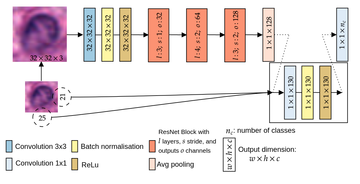
Figure 2: Small image ResNet-18 with possible concatenation of image size. (No SDCL here)
Datasets
TNBC – New extension – Small dataset
We extend the TNBC dataset by adding cell type as well as 3 new images from brain tissue. To note the brain tissue is not used in the paper.
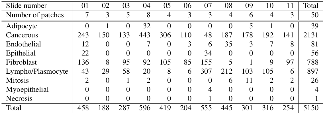
Table 1: Nuclei types within each sample of the TNBC dataset
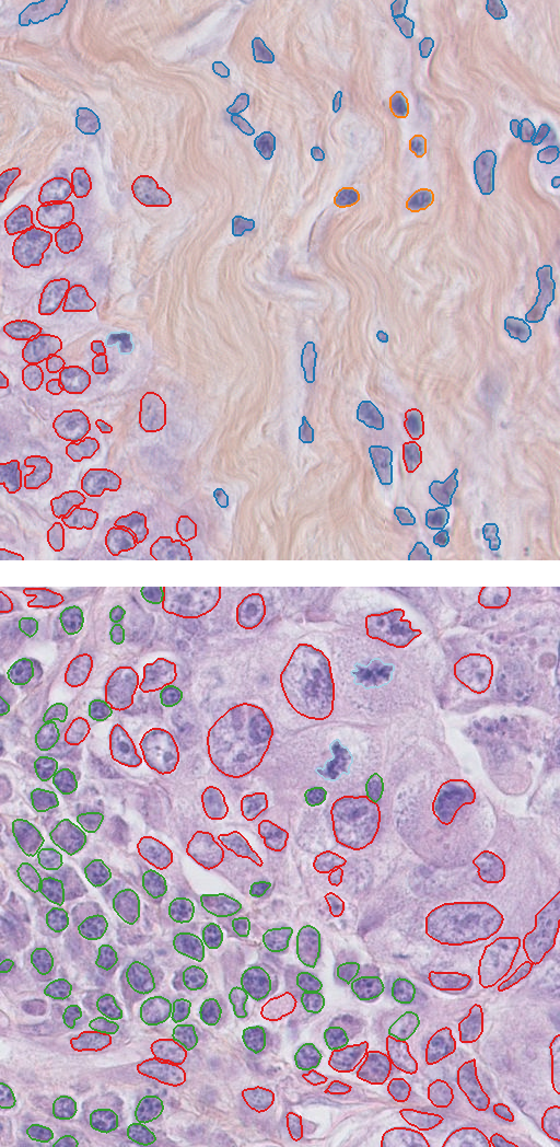
Figure 3: Samples from the TNBC dataset
After splitting the dataset into train and test, we have $3,259$ train samples and $759$ test samples.
CoNSep – Medium dataset
After splitting the dataset into train and test, we have $15,555$ train samples and $8,777$ test samples.
PanNuke – Large dataset
After splitting the dataset into train and test, we have $122,117$ train samples $67,627$ test samples.
Results – Ablation study
We perform 20 repetitions of each model and report the results in the following table.
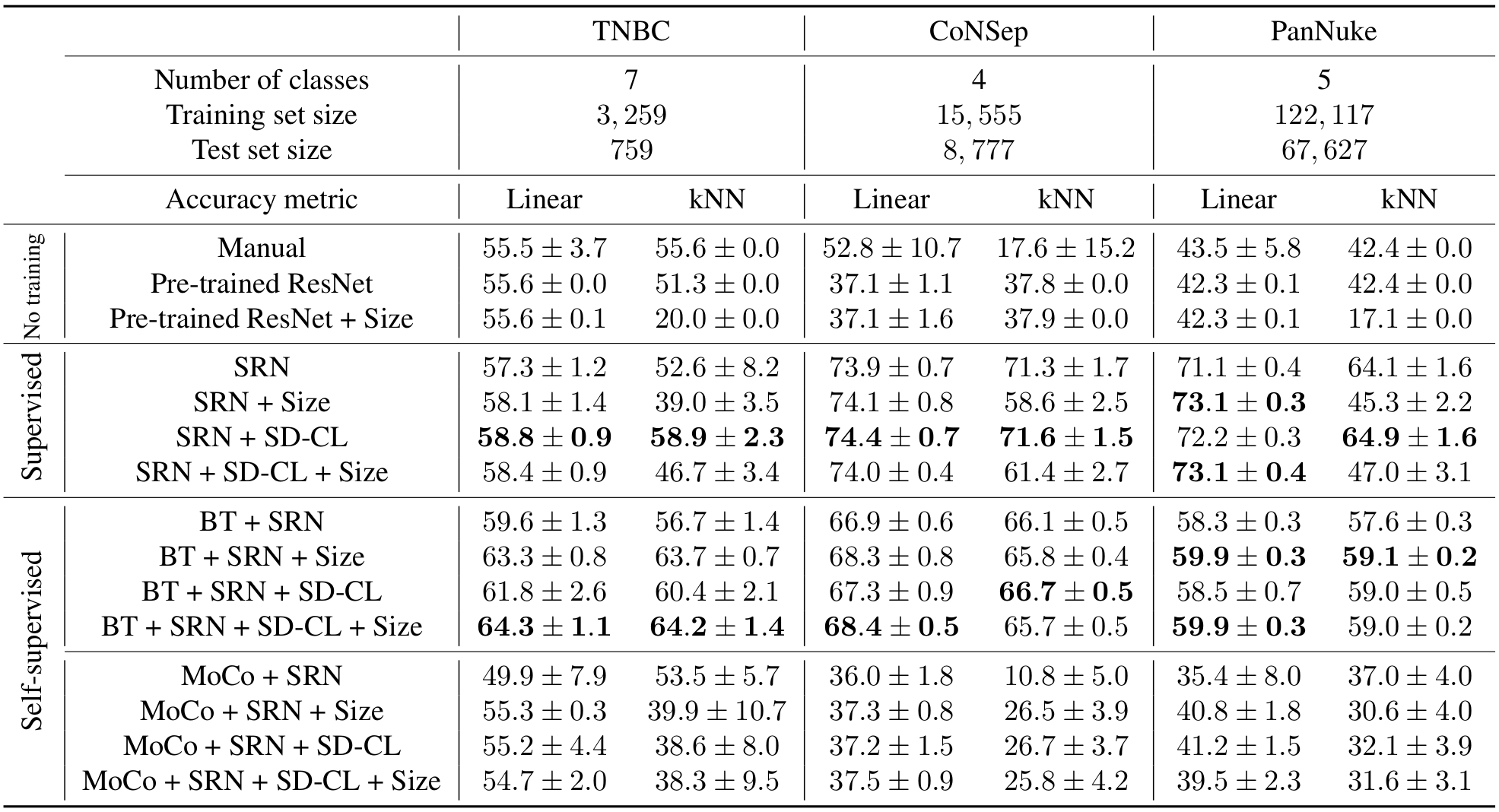
Table 2: Benchmark and results
On two good performing networks, we show the learned weights of the first convolution layer and of SDCL.
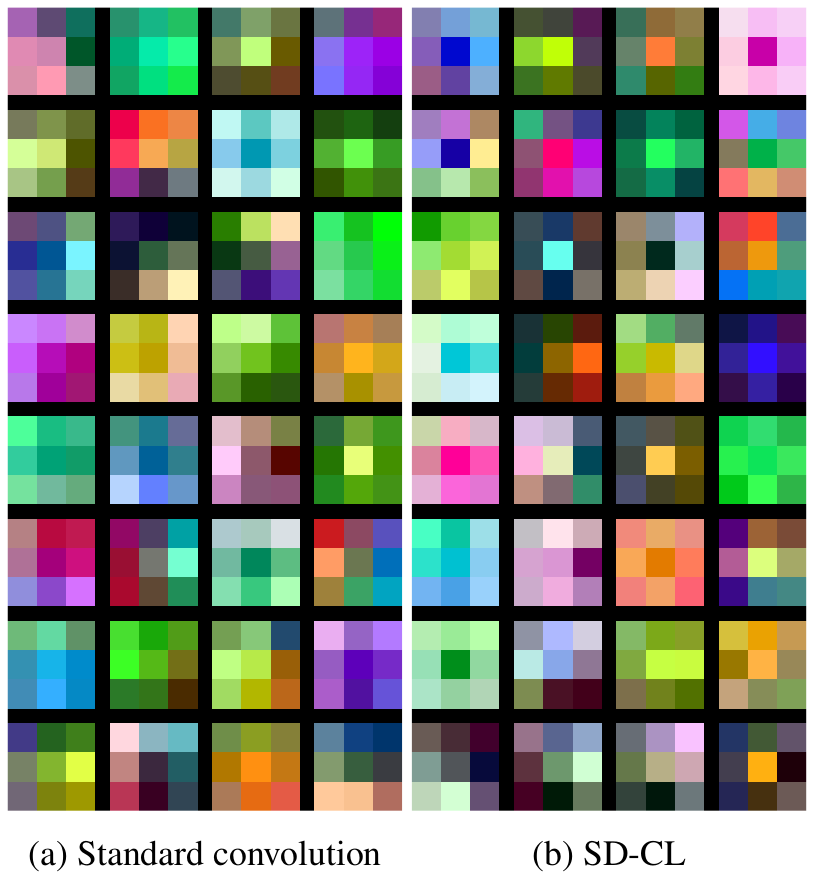
Figure 3: Visualisation of the learned weights in the first layer of the ResNet-18
Conclusion
We compare hand-designed features, pre-trained models, supervised models and self-supervised models on three nuclei type datasets that range from small to large samples size. In this benchmark, we show the effectiveness of differently produced encodings. The self-supervised learning Barlows-twins model ahead in the low sample setting and the supervised learning ahead in the large sample setting. Moreover, we presented a new convolutional layer for extracting features dependent on the scale. In addition to accounting for the scale, this layers impacts positively the performances and shows similar weight introspection to the standard convolution layer. In the spirit of open science and reproducibility, the cell type extension dataset for TNBC and the code are made publicly available.
Data and code availability
The TNBC segmentation dataset is available here. The extended TNBC classification dataset is here. The CoNSeP segmentation and classification dataset is available on the website of the corresponding laboratory here. The PanNuke segmentation and classification dataset is available on the website of the corresponding laboratory here. The code for MoCo used the lightly package and the code for BT was inspired from GitHub. In addition methodological developments, for the sake of reproducible research and open science, we make the code for all experiments publicly available in the following Github repository ScaleDependentCNN.
